GeneScreen

Walk-through guide

Note: This program requires the Microsoft .NET framework version 2 or later to be installed on your computer.

This walk-through of the program uses the sample files in the GeneScreen_sample_files folder. There are five main sections to this guide:

1. The creation of reference sequence files
2. Searching for mutations/SNPs in multiple ABI files
3. Searching a sequence for heterozygous indels
4. Exporting data to a file or database (LOVD)
5. Analyzing a single sequence file

1. Creating reference sequences

1. In this Section:
2. 1.1. Importing mRNA sequence information
3. 1.2. Importing genomic sequence information
4. 1.3. Primer design
5. 1.4. Choosing the PCR products

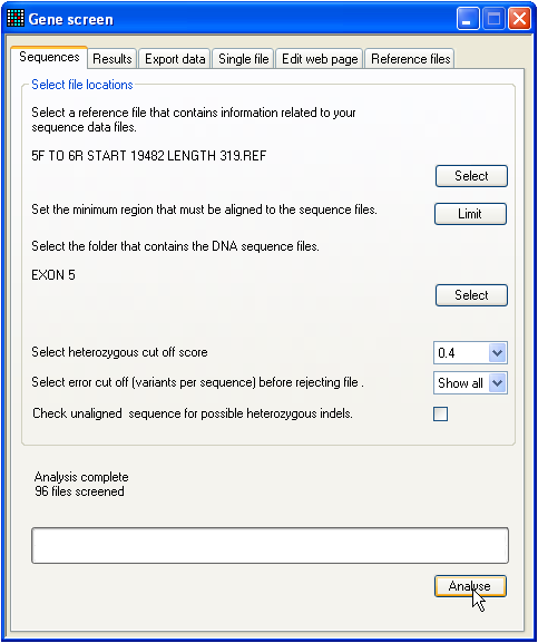
Figure 1: The start-up screen.

When the GeneScreen program starts, the tab for analysis of sequences is initially shown (Figure 1). This is because this tab will most likely be used multiple times for analysis of ABI sequences. The creation of a set of reference files, in contrast, will in general be done only once.

To create reference sequences, click the Reference files tab at the right of the tab-bar (Figure 2).

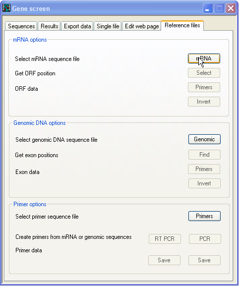
Figure 2: Reference sequence production window

Reference sequences can simply be plain text sequence files. However, if you wish to screen a gene whose cDNA and genomic sequences are both available, you can make reference files that contain additional information on the open reading frame, exons/introns and protein sequence.

1.1. Importing mRNA sequence information

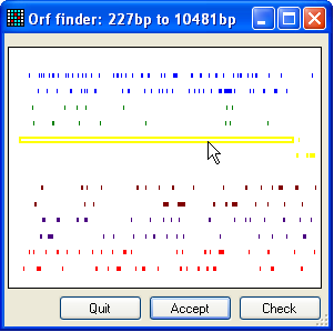
Figure 3: Selecting the correct ORF

To create an annotated sequence file, press the mRNA button (Figure 2) and select the file in the BRCA2 source sequences folder called cDNA.txt. Then, press the “Get ORF position” Select button. This will screen the sequence for open reading frames (Figure 3). The window in Figure 3 displays six different sets of coloured lines, representing the possible reading frames. Only the forward frames are available for selection. If the desired ORF is on the reverse complement strand, close the window and press the Invert button (Figure 2, three buttons below mRNA) and then press the Select button again.

To select an ORF, place the cursor over the appropriate line (in Figure 3 it's the longest (yellow) line) and click the left mouse button. The selected line will then become hollow. If you want to check that you indeed have the correct ORF, press the Check button, whereupon the window in Figure 4 will be displayed. This form allows you to select options for generating an annotated text file showing the protein and mRNA sequence alignment. The format of this output file will change according to the options selected from the form, and will be shown in preview form in the bottom left of the window. (The sequence displayed is a generic one, not the actual selected sequence.) To generate the output file, press the Create button. To accept the ORF, close the window shown in Figure 4 (if opened) and confirm by clicking the Accept button (Figure 3).

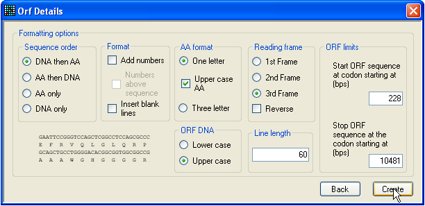
Figure 4: Checking the ORF

If you do not wish to include any genomic sequence in the reference files, you can create the reference sequences now, by either designing or importing a list of primers that you intend to use in the PCR amplification/sequencing of the mRNA. This process is the same as for creating files with genomic sequence information, so this step is illustrated later.

1.2. Importing genomic sequence information

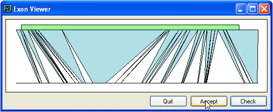
Figure 5: Finding exons

Just as reference files may be created without genomic sequence information, they may be created without mRNA sequence information, by omitting the steps in Section 1.1. To import a genomic sequence, press the button labelled Genomic (Figure 2) and select a plain text sequence file corresponding to the genomic region (including 5'-UTR, 3'-UTR, introns and exons). For the purposes example, use the file called Genomic.txt. To find the positions of exons, press the Find button (only if an mRNA sequence has already been added). This will display the window shown in Figure 5. If you get a message that says no alignment was found, press the Invert button (three buttons below the Genomic button) and try again.

The upper green box represents the position of the ORF within the mRNA, while the blue triangles show the regions of sequence alignment between the mRNA (upper line) and the genomic sequence (lower line). To check the alignment, press the Check button and save the alignment to disk. (To reduce the size of the alignment file, unaligned intronic and intragenic sequence is removed, apart from short regions that flank the exons.) If the alignment is correct, press the Accept button.

1.3. Primer design

Once you have created the alignments, the relevant Primers buttons shown in Figure 2 will be enabled, allowing you to design primers. However, if you wish to design primers using a different software package, you can alternatively import primers as plain text, in the tab-delimited format used in the Primers.txt file. To import primers, under Primer options press the Primers button (third from the bottom). Or, to design primers using GeneScreen, press one of the other Primers buttons (either under mRNA options or Genomic DNA options) which will cause the following form to be displayed:

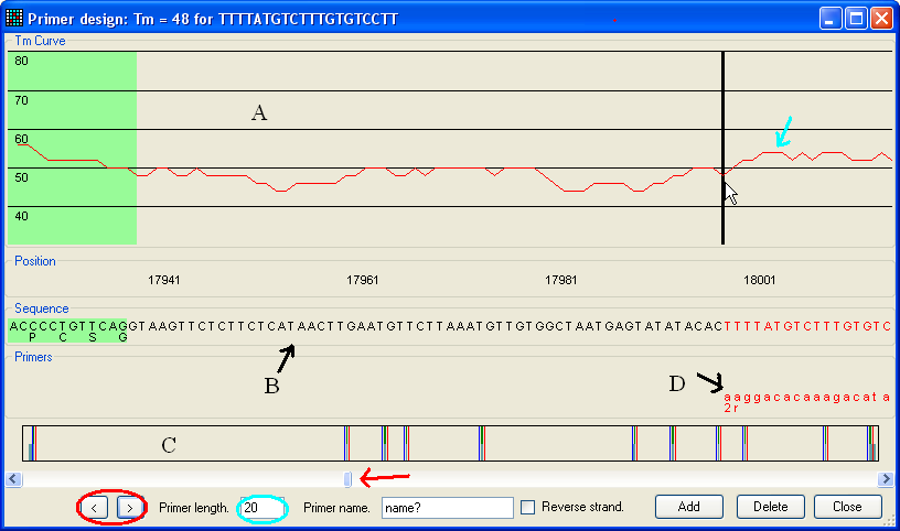
Figure 6: Primer design

The primer design window contains three regions.

The upper region (A in Figure 6) shows the calculated T_m for primers (red line, indicated by blue arrow) of the currently selected length as shown in the text box (blue ellipse).

The middle region (B) shows the sequence currently in view (including any protein translation where appropriate) and the lower panel (C) shows a scaled graphic of the total genomic region. In these panels, green areas represent protein-coding regions and blue areas indicate 5'- and 3'-UTR sequences. The lower panel shows all the exons etc. (In this image the exons are difficult to see.) The positions of forward and reverse primers are shown by blue and red lines respectively.

The user can navigate along the sequence either using the scroll bar (red arrow) or the < and > buttons (red ellipse). The latter buttons move the display to the next sequence feature i.e. an intron/exon splice site, start/stop codon or start/end of the mRNA.

To create a primer, place the cursor over the primer site and click the left mouse button. The chosen primer’s sequence and T_m will be displayed in the title bar of the window, and the corresponding sequence in panel B will be coloured red. The primer length can be altered using the text box highlighted with a blue ellipse in Figure 6. After entering a name for the primer, tick the box labelled “Reverse strand”, if the primer is for the reverse strand, and finally click the Add button. The chosen primer will now appear in the Primers panel (labelled D in Figure 6); as in panel C, forward primers appear in blue and reverse primers in red.

To save the primers, press the Close button.

1.4. Choosing the PCR products

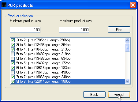
Figure 7: Selection of PCR products

Once primers have been entered, either selected as described above or imported from a file, the set of PCR products can be chosen, which it is desired to convert into reference files. To do this, click either the RT PCR or PCR button (Figure 2). The RT PCR option will look for PCR products within the mRNA sequence, while the PCR option screens the genomic sequence. Selecting one of these buttons generates a form of the type shown in Figure 7: initially, the large text box will be empty.

Adjust the minimum and maximum product size values, so that excessively long or short products are ignored, and then press the Find button. The window will then display a list of possible PCR products. From this list, select the products that you wish to convert into files, and click Accept. The form will close and the Save button will be activated. Pressing this button will prompt the user to select a folder to save the reference files to, and then generate these files, along with a file containing the names and sequences of the primers used to create these files.

2. Searching for mutations or SNPs in multiple ABI files

1. In this Section:
2. 2.1. Selecting sequences and analysis parameters
3. 2.2. Interacting with the Results grid
4. 2.3. The View window
5. 2.4. The Edit form
6. 2.5. The Annotate form
7. 2.6. Genotyping a SNP
8. 2.7. Analysis of rejected sequences

2.1. Selecting sequences and analysis parameters

To search a number of ABI trace files (*.AB1) for mutations, place them all in a single folder and create a reference file. If you choose to use an unannotated file, the sequence should have a maximum length of 1000 bp. Select the Sequences tab (Figure 1) and use the upper Select button to pick the desired reference file. Next, use the lower Select button to pick the folder containing the trace files. This folder should be on a local hard disk, and not a network drive, since the operating system may restrict the program’s access to these files. Select the “heterozygous cut-off” value; this refers to the ratio of the two allelic peak heights at a heterozygous position. If the trace files have a high background, this cut-off value should be increased in order to reduce the number of false positives.

Also, through the next drop-down listbox on the Sequences tab (Figure 1), it is possible to set a maximum permitted number of sequence variants per trace. If this number is exceeded, that trace file is deemed to have “failed” (see Section 2.7).

If a sequence cannot be aligned to the reference file, it can be checked for the presence of a heterozygous indel. To use this option, tick the last checkbox on the Sequences tab (Figure 1).

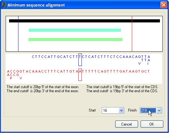
Figure 8: Selecting a region of interest for mutations

To restrict sequence variant highlighting to a particular region of the reference file, press the Limit button, whereupon the window shown in Figure 8 will appear. The solid black bar represents the reference sequence, while the pale blue and green bars represent any exons or protein coding sequences (respectively) in the reference file. The selected region lies between the blue and red vertical lines, the positions of which can be moved either by positioning the cursor over the image and pressing a mouse button, or by changing the base pair positions selected in the list-boxes at the bottom right of the window. The chosen region is accepted by pressing the OK button.

Finally, (returning to the Sequences tab) press Analyse. The progress of the program will be shown in the progress bar below the Analyse button. When all the trace files have been screened, the number of files that were aligned will be displayed in a message above the progress bar on the Sequences tab (Figure 1).

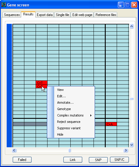
Figure 9a: The results data set

When analysis is complete, the program will switch to the Results tab (Figure 9a). Unlike the other tab views, this can be resized (Figure 9b) to allow the user to see more data.

Figures 9a and 9b show the appearance of the grid after analysis of the sample files contained in the folder BRCA2 exon 23, using reference file 23f to 23r start 73141 length 269.ref (also in this folder).

In this display, each row represents a file, and each column a basepair position that contains at least one (possible) mutation in the analysed sequences. The number at the top of each column identifies the position of the (possible) mutation within the reference file. If you already chose, as described above, to define a region of interest, any sequence variant located outside the chosen region will ignored.

To identify the file represented by each row, move the cursor over the blue bar at the left of the window. If the number of rows or columns exceeds the viewable area of the form, the grid can be moved using the vertical and horizontal scroll bars, at the right and bottom of the grid. Each cell in the grid is colour coded:

Moving the cursor over the cells in the data grid causes a small window to appear, displaying additional information about the underlying nucleotide, such as any predicted amino acid change. Clicking the left mouse button invokes a floating menu, as shown (Figure 9a), from which each menu item causes a separate window to be displayed, as described below

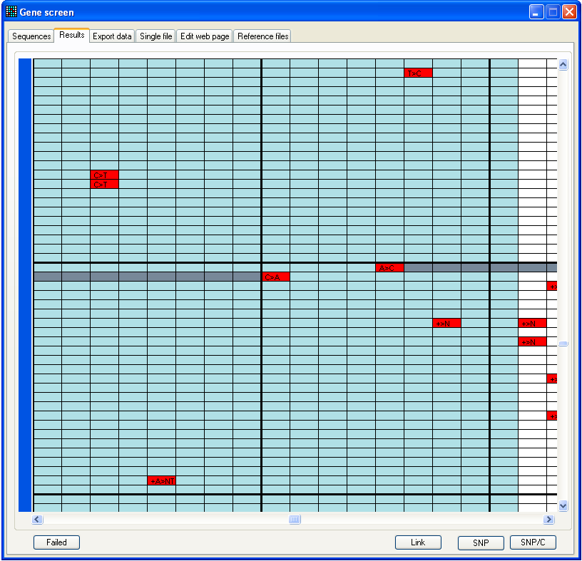
Figure 9b: Results tab window is resizable

This figure shows the appearance after analysis of the files in the folder BRCA2 exon 23, using reference file 23f to 23r start 73141 length 269.ref, also in this folder.

2.2. Interacting with the ‘Results’ grid

The program has a number of features designed to speed up the screening of large numbers of sequences for possible mutations. These functions fall into two main categories:

1. Dynamic display of the underlying trace data
2. Updating the Results grid to display the action taken on a sequence variant

2.2.1. Dynamic display of trace data

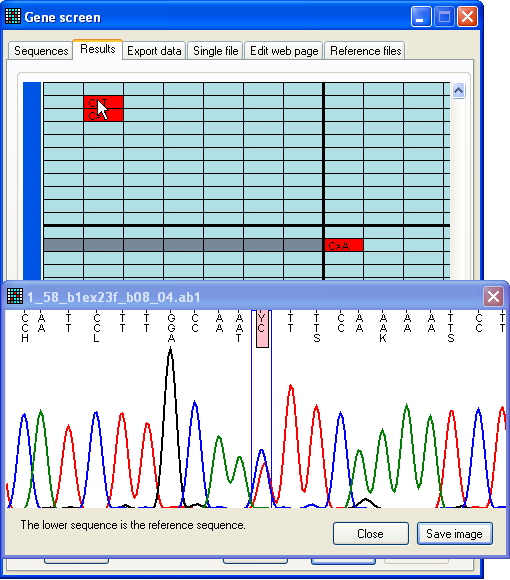
Figure 10: Dynamic display of sequence flanking a possible mutation

Pressing the SNP button (to the lower right on the Results tab) displays the View window (Figure 10). This window is described in greater detail below; however, in this mode, the image in the window is dynamically linked to the cursor position over the Results grid. As the cursor moves from one cell to another, the image in the View window thus changes to display the variant position and flanking sequence corresponding to that cell.

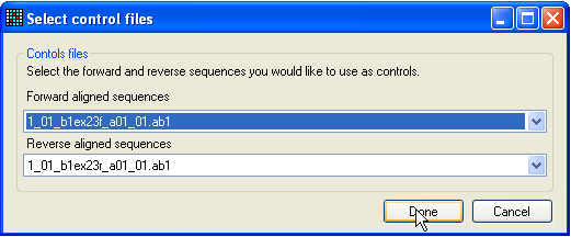
Figure 11a: Selecting control traces to compare with the query sequence

Alternatively, if you also want to compare the variant position to a corresponding control sequence, click SNP/C. This button operates in a similar manner to the previous one, but before the dynamically linked View window is displayed, a control sequence must be selected (Figure 11a). Typically, one would select both a forward and reverse control sequence, but it is possible to select just one trace.

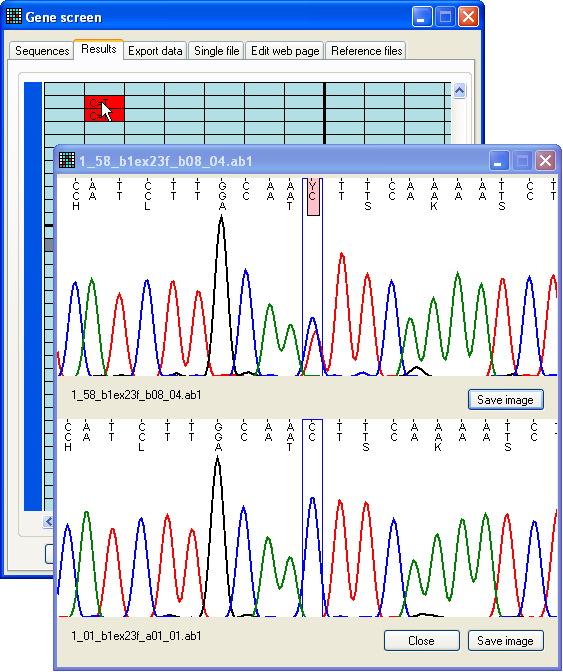
Figure 11b: Dynamic display of a possible mutation compared to a control trace

As before, the trace shown as the upper image (Figure 11b) is now linked to the position of the cursor, while the lower image displays the control sequence trace at the same position. (If you selected both forward and reverse control sequences, the correct control sequence, matching the direction of the test sequence, will be displayed as the control image.)

2.2.2. Editing the ‘Results’ grid to display tasks performed on a mutation

In the Results grid, the sequences are arranged in alphabetical order. Typically, therefore, if a patient ID or name is the first variable part of the file name (e.g. ID2323_Rev_Brac1_exon23.ab1 or exon1_AFM_f.abi), the list will alternate between forward and reverse sequences for each individual. However, if the sequence direction is placed before the patient ID in the file name (e.g. Brac1_exon23_Rev_.ID2323ab1 or exon1_f_AFM.abi), all forward sequences will be grouped together, followed by the reverse sequences. Finally, if the first variable part of the file name is related neither to the sequence direction or patient ID, the trace will appear to be randomly placed in the Results grid.

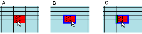
Figure 12: True mutations appear as pairs in alternating forward and reverse reads

Figure 12 shows a region of a typical grid in which the sequences alternate between forward and reverse reads for each individual. Two red cells indicating possible mutations appear together, suggesting that they represent a true sequence variant, seen both in forward and reverse direction. To confirm that they do belong to the same individual, it is possible simply to view the underlying sequence data (as shown above) and read the file names, shown in the form title-bar. Alternatively, clicking the Link button (centre bottom of the grid view in Figure 9a) draws a blue box around the matching pairs. If forward and reverse sequences alternate, one box containing both variants is drawn (B). Otherwise, a separate blue box is drawn around each matched variant. Since this function depends on correct recognition of matching forward and reverse name pairs, with some naming schemes for data files it may not work correctly. If you decide to annotate and export the variant, a light green rectangle is drawn to the left of the cell (C).

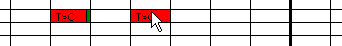
Figure 13: Marking a sequence variant as "dismissed"

When analysing a large number of sequence files, it is possible to forget which variants have been examined and what action was taken. To remedy this, the grid may be annotated as the underlying data are being viewed. The simplest annotation is to mark a variant as an artefact, by simply placing the cursor over the cell and pressing the ‘m’ key. This marks the cell with a dark green rectangle, indicating that it has been viewed and the sequence variant has been disregarded (Figure 13).

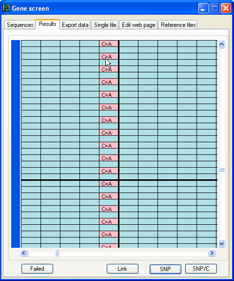
Figure 14: Suppressing all instances of a selected variant

If your sequence contains a common non-pathogenic SNP, or is subject to a sequence-specific artefact, it is possible to suppress all instances of the same sequence variant. To do this, place the cursor over a cell that exhibits the variant, and type ‘Ctrl-S’. Any variants at the same position in the reference file, that were sequenced in the same direction and exhibit the same sequence variant, will be redrawn in pink rather than red.

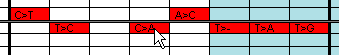
Figure 15: Ctrl-R to manually reject an aligned sequence

If the program managed to align a low quality sequence to the reference file, it is still possible to manually reject the file. To do this, either press ‘Ctrl-S’ or left-click on the row and select Reject. Manually rejected sequences are then identified by a thin grey line running along the top of the row. If you change your mind, repeating the action will “de-reject” the sequence and the grey line will be replaced by an orange one.

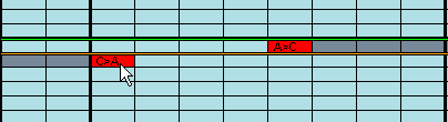
Figure 16: Manual rejection of an exported indel

Similarly, if you export a heterozygous indel, the sequence will be identified by a green line along the top of the row. If you change your mind, the heterozygous mutation can be deleted by left-clicking the row and selecting Delete; the green line will then be replaced by an orange one.

2.3. The ‘View’ window

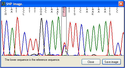
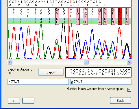
Figure 17: Flanking sequence around a possible mutation

The View window displays the sequence flanking the mutant nucleotide (Figure 17). The image includes three lines of text; the upper shows the trace sequence, the middle and lower show the reference nucleotide sequence and its translation (where applicable). Positions where the trace and reference sequences differ are highlighted by pink rectangles, and the blue box identifies the nucleotide under scrutiny.

2.4. The ‘Edit’ form

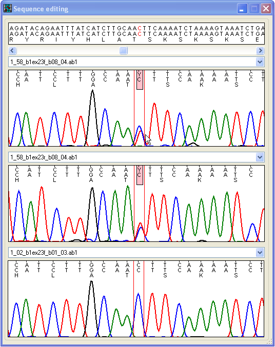
Figure 18: Compare different trace files and edit base-calling

The Edit form can be accessed either by clicking on a cell in the data grid or via the Edit button at the bottom right of the Results tab (Figure 9). The Edit form contains four regions (Figure 18). The lower three display trace file data, while the upper panel shows the relevant reference file genomic, exonic and protein sequences. The sequence displayed in each of the lower panels can be changed by selecting a different file name from the drop-down list above each panel. The format of each trace image is the same as that used in the View window described above. However, unlike the View window, it is possible to navigate along the sequence, using the scroll bar beneath the upper text panel. The nucleotide displayed in red text in the top panel corresponds to the position between the two red lines in the three trace image panels.

It is also possible to edit the base calling for each trace file using this window. To make a visual assessment of the validity of a possible mutation, display the forward and reverse sequences from an individual in the top two trace panels and a reference sequence in the lowest panel. If it appears that the mutation is either a sequencing artefact or base-calling error, the sequence can be edited by placing the cursor over the aberrant base, clicking the left mouse button, and selecting an option from the floating menu (Figure 19).

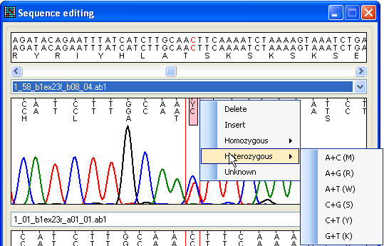
Figure 19: Editing the trace sequence

To change or delete a nucleotide, place the cursor over that nucleotide. To insert a nucleotide, click on a position in the space between two residues and select the Insert option. This will insert an N in the sequence, which can then be reselected and edited to the desired residue. After editing a sequence, the underlying data are realigned once the edit form is closed, whereupon the mutation data grid will be revised.

2.5. The ‘Annotate’ form

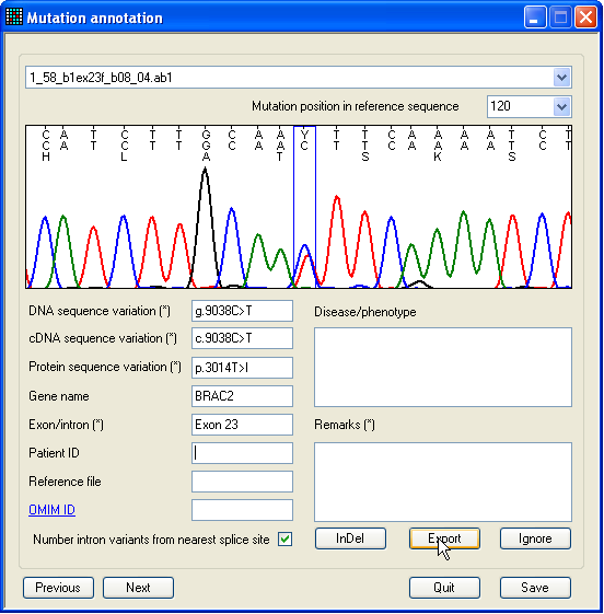
Figure 20: The single-nucleotide mutation annotation form

Once the putative mutations displayed in the data grid have been checked, they can be exported, either to a text file, a web page or an import file for the LOVD mutation database. However, before this can be done, the mutation must be selected for export, and (optionally) annotated.

To mark a single-nucleotide mutation for export, select the Annotate option (Figure 9a), to display the form shown in Figure 20. This contains an image of the selected region, in the same format as in the previous two forms. The form also contains text boxes that allow annotation of the mutation. Those boxes describing the sequence variant itself are automatically filled by the program, but can be user-edited. Once the annotation process is complete, click Export to mark the sequence variant for export. (If you later change your mind, click Ignore.) A new sequence can be selected using the drop-down list-box above the image panel, while the displayed nucleotide position can be selected using the list-box beneath this. (Only positions that are linked to a mutation are selectable in this drop-down list.) Alternatively, you can cycle through the sequence variants by pressing the Previous or Next buttons.

To annotate and export heterozygous indels, or complex mutations that affect more than one nucleotide, select Complex mutation > Annotate (Figure 9a); this displays the Annotate heterozygous indels form described in Section 3.

2.6. Genotyping a SNP

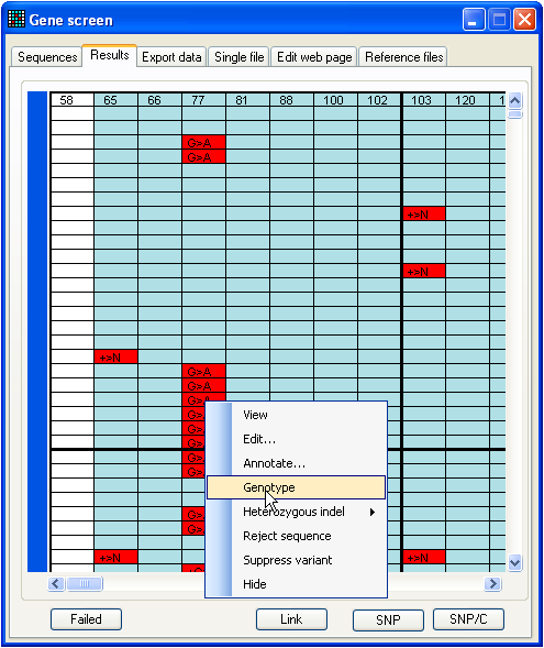
Figure 21: Saving genotype data

To demonstrate the Genotype function, analyse the data in the BRCA2 SNP folder, using the reference file 2f to 2r start 9785 length 250.ref (also in the same folder). This folder contains 190 files, and should generate the data grid shown in Figure 21. When the data are viewed, a number of polymorphic nucleotide positions are identified. To analyse the genotypes of the files at nt 77, left-click a cell in the corresponding column, select Genotype from the floating menu, and then save the data as a web page or text file. If you select “web page”, an additional folder will be created to contain the images needed by the web page.

Figure 22 shows the bottom of the resulting web page, with the data from the last two trace files and a summary of the allele frequencies for the set of sequences.

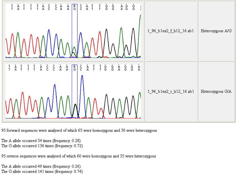
Figure 22: The bottom of a genotype web page

When creating a genotype webpage, GeneScreen counts the numbers of heterozygous and homozygous sequences in the sequence trace folder. Since the scoring of some variants is adversely affected by differences in context-dependent dideoxynucleotide incorporation, the allele frequencies for forward and reverse sequences are shown separately. The rationale for this is illustrated by Figure 22, in which the forward sequence (upper image) displays a reduced peak height of the G allele compared to the A. In some situations, this may cause the program to disregard a heterozygous sequence variant (if the difference in peak heights is greater than the heterozygous cut-off limit).

2.7. Analysis of rejected sequences

Sequence files can be rejected on a number of criteria:

1. The sequence could not be aligned to the reference sequence.
2. The alignment did not span the entire region of interest.
3. The sequence contained more than a preselected number of sequence variants.
4. The user rejected the sequence manually.

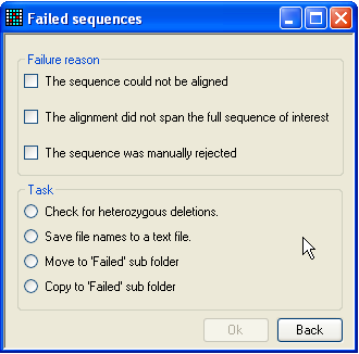
Figure 23: The ‘Failed sequences’ form

The Failed sequences form allows you to list the failed sequences, screen them for heterozygous indels, or move/copy them to a different directory.

Pressing the Failed button at the bottom left of the Results grid (Figure 9a) displays the Failed sequences form (Figure 23). This allows the user to perform certain actions on the rejected files. The files are grouped together, depending on the reason they were rejected. To select which group(s) to work with, tick any or all of the three boxes in the upper panel. (Note that files which failed by exceeding the permitted number of sequence variants (criterion 3 above) are included in the middle category (The alignment did not span the full sequence of interest). The task you wish to perform is then selected from the radio buttons below, and is executed by pressing OK. If the option to move or copy the failed files to the Failed folder is selected, this folder will be created within the trace file folder (and named Failed). Note that if you do move the files, then the program will no longer be able to copy the files or check for heterozygous indels (see below).

2.7.1. Rejected sequences and heterozygous indels

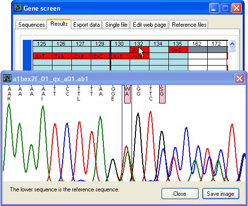
Figure 24: Apparent sequence failure due to heterozygous indel

Since trace files that contain heterozygous indels can be very difficult to base call and align to the reference sequence, they often appear as low quality sequences. This means that all failed sequences should be checked for heterozygous indels. This can be done either by using the Failed sequences form described immediately above, or by left-clicking on the row linked to the failed sequence and selecting Complex mutations > Annotate. This will open the form shown in Figure 25. If you arrive at this window via the Failed sequences form, all the sequences will already be available via the list-box (below the “Select the trace file that contains the InDel” label). It must be noted that the program re-reads the data file when analysing the sequence for indels, and so it will fail if you have moved the apparently failed source files to a different folder during earlier analysis (see Analysis of rejected sequences above). Further information on indel analysis using this form follows in Section 3 below.

3. Analysis of heterozygous indel mutations

Due to the difficulty of automatically distinguishing sequences containing heterozygous indels from those that happen to have short regions of high quality data followed by low quality data, trace files must currently be analysed for heterozygous indels one at a time. This limitation will be resolved in future versions of GeneScreen.

a.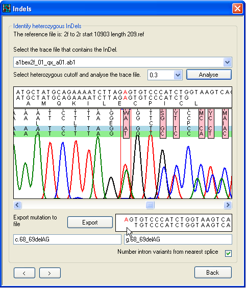

b.

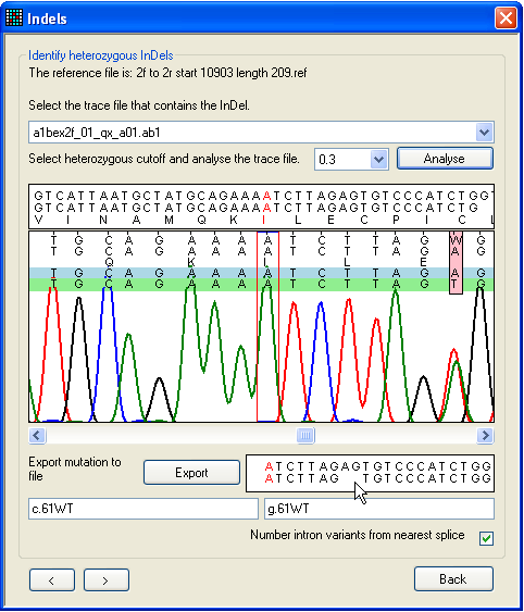
Figure 25: Screening a sequence for heterozygous indels

To screen a file for heterozygous indels or other complex mutations, use the form shown in Figure 25. This can be reached via the Failed sequences window, left-clicking on the grid (Figure 24), or directly from the Single file tab.

First, pick the trace file for analysis using the drop-down list. Next, click Analyse, and use the horizontal scroll bar (beneath the trace image panel) to navigate along the sequence. The text box below the scroll bar shows the sequences from the trace file and reference file; ambiguous positions are resolved by subtracting the reference sequence from the trace sequence. (If the trace sequence is the reverse complement of the reference file, this box has a pale yellow background.) The program assumes that one allele matches the original reference sequence; this allele is shown shaded blue, while the deduced other allele (result of subtraction) is shaded green.

In Figure 25a, a heterozygous 2-nt deletion within the sequence AGAG is shown. The first ambiguous nucleotide after the deletion is visible as a pink rectangle. The resolved sequences for the two alleles are displayed in the text box at the bottom right of the window and the mouse pointer is indicating the position at which the dinucleotide is deleted on one allele. As in other windows, the red nucleotide in the text box corresponds to the position between the red lines in the trace image panel. In Figure 25b, the red highlighting point has been moved to the point at which the deletion occurs, and the nomenclature for the deletion is displayed in the bottom text box.

If the program fails to align and resolve a suspected indel, adjusting the heterozygous cutoff value (next to the Analyse button) may resolve the problem.

a.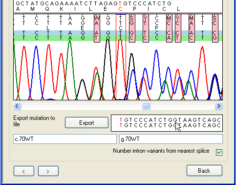

b.

Figure 26: Editing the base calling on the Indels tab

Since it can be difficult to accurately base-call a sequence that follows a heterozygous indel, the program allows manual editing of the sequence in the trace panel, in the same way as in Figure 19. Figure 26 illustrates the difference editing can make. In Figure 26a (before editing) the mouse arrow shows the position of a spurious extra Y nucleotide that has been incorrectly inserted due to the mobility shift between the C and T peaks. In Figure 26b the extra nucleotide has been manually deleted, with the result that the alignment of the deduced allelic sequences in the lower text box is resolved. The program can now correctly annotate this heterozygous mutation and display the aligned allelic sequences beyond the deletion point.

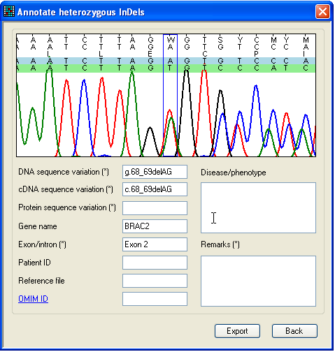
Figure 27: The Indel annotation form.

As before, to export this variant, click Export to display the annotation form (Figure 27). This form is very similar to the one shown in Figure 20 and works in the same way, except that only one file can be viewed and it is not possible to navigate along the sequence. This form can only export the nucleotide highlighted in red on the Indels window. The action performed by clicking Export depends on how you arrived at the Indels window:

– If via the Single file tab, the mutation is exported according to the options selected on that tab (Figure 30).

– If via the Failed sequences window or from left-clicking on the grid (Figure 24), the mutation data are saved along with all other mutations, and can later be exported using the Export data tab (Section 4, Figure 28).

4. Exporting sequence variants

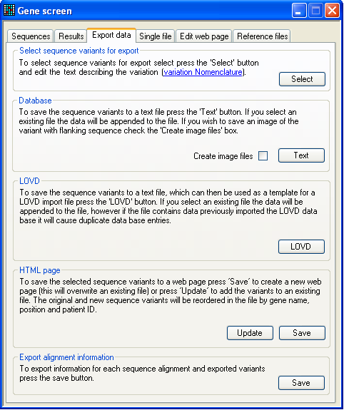
Figure 28: The Export data tab.

This tab allows you to export the sequence variants to either text files, web pages or the LOVD database (Figure 28). If no mutations have been marked for export, all buttons will be disabled apart from the first, labelled Select. Pressing Select will display the annotation form (Figure 20), enabling you to annotate the sequence variants. For help in situations in which a mutation is of a complex type that the program cannot resolve, there is also a hyperlink to the DNA / protein mutation nomenclature web site next to this button.

The first data export option Database creates a tab-delimited text file that contains the annotation information as well as the sequence variant. (If you select an existing file to save to, the data will be appended to the end of that file.) This file can be viewed and edited in a plain text editor or in a spreadsheet program.

The LOVD option saves the data to a file that can be used as a template to create a database import file for the Leiden Open Variation Database, LOVD. Since there is no standard field format for this database, it is not possible to create a file that can be directly imported into LOVD. However the file is very similar to that needed by a standard installation of LOVD.

The HTML page option creates a web page that contains all the variants marked for export, and orders them by gene name, nucleotide position in the reference file and patient name. If an existing file is selected, the original file is read and its data combined with the current data to produce a new file with all the sequence varants in the correct order. This allows the web page to be used as static web page and as a dynamic database.

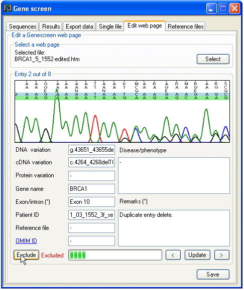
Figure 29: The Edit web page tab.

A mutations web page can be edited by using the Edit web page tab. First load the desired web page using the Select button. The program will then read the web page and present the mutation data one row at a time, as shown in Figure 29. Use the buttons labelled < or > to move through the rows. The current position of the mutation within the web page is indicated by the progress bar next to the < button. All the data fields can be edited, and the corrections saved by pressing the Update button. However, note that if you move to a different mutation without pressing Update, any changes will be lost.

5. Analysing single files

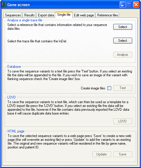
Figure 30: The Single file tab

For quick analysis of a single ABI sequence trace, without needing to work with the grid interface, the Single file tab may be useful. First select the reference file and test (.AB1) file and then press Analyse. This will open the Indels window which can be used to analyse the sequence as described in Section 3. Since data analysis initiated via this tab is separate from that performed through the Sequences and Results tabs, different data may be analysed simultaneously through the Single file tab. However, if this is done, to export a mutation you must use the Export options on the Single file tab and not those on the Export data tab.